Testing the "Internal Bar Strength" strategy

Looks more or less OK.

The Idea

A few days ago, I came across this piece by Sofien Kaabar on the “Internal Bar Strength” indicator, on his All About Trading! Substack.

Very simple concept using this indicator:

𝐼𝐵𝑆=(𝑐𝑙𝑜𝑠𝑒−𝑙𝑜𝑤)/(ℎ𝑖𝑔ℎ−𝑙𝑜𝑤)

With these simple trading rules: Long entry when IBS<0.2 and Exit when IBS>0.8

Results look pretty interesting in the TradingView platform. It looks like an interesting strategy to trade with US equity index futures, to avoid the “wash sales tax” when trading ETFs (for US citizens/residents, due to the higher trade frequency), and to reduce trading costs.

Analysis

Let’s expand Sofien’s analysis to a lot of markets, beyond S&P500, and check how it performs. Here’s a market universe of CSI Data symbols with categories by yours truly.

symbol.frame=data.frame(
  symbol=c('MES','MNQ','M2K' ,'MYM' ,'FNG',
           'A50','SIN','JTM',
           'FXP','FDX',
           'C2','W2','S2','SM2','BO2',
           'EMA','COM','BL2',
           'KC2','SB2','CT2','LB','LBR','CC2',
           'LCC','LRC','LSU',
           'GC2','SI2','PA2','PL2','HG2',
           'LC','LH', 'FC',
           'CL2','RB2','NG2','HO2',
           'VX','FVS',
           'EBL','TY'
           ),
category=c('US.EQ','US.EQ','US.EQ','US.EQ','US.EQ',
           'ASIA.EQ','ASIA.EQ','ASIA.EQ',
           'EUR.EQ', 'EUR.EQ',
           'US.GRAIN','US.GRAIN','US.GRAIN','US.GRAIN','US.GRAIN',
           'EUR.GRAIN','EUR.GRAIN','EUR.GRAIN',
           'US.SOFT' ,'US.SOFT', 'US.SOFT','US.SOFT','US.SOFT','US.SOFT',
           'EUR.SOFT','EUR.SOFT','EUR.SOFT',
           'US.METAL','US.METAL','US.METAL','US.METAL','US.METAL',
           'US.MEAT' ,'US.MEAT','US.MEAT',
           'US.ENERG','US.ENERG', 'US.ENERG','US.ENERG',
           'VOLA','VOLA',
           '10YBOND','10YBOND')
)

Now let’s compute performance for each market without compounding, and sizing by inverse volatility for apples-to-apples comparison; since each future has a different contract size and natural volatility. To see if we can find some patterns…

BA=fGetFuturesBA(symbol.frame$symbol)%>%
  inner_join(symbol.frame,by='symbol')%>%
  group_by(symbol)%>%
    arrange(date)%>%
    #Indicators
    mutate(
      annvola=roll_sd(log(close.r/lag(close.r)),30)*16*100,
      ibs=(close.p-low.p)/(high.p-low.p)
    )%>%
    #Signal
    mutate(signal=case_when(
      ibs<0.2 & lag(ibs)>=0.2 ~ 1,
      ibs>0.8 ~ 0,
      T ~ as.numeric(NA)
    ))%>%fill(signal)%>%mutate(signal=replace_na(signal,0))%>%
    #Sizing  
    mutate(
           #Position sizing such that you lose 5% of account
           #when 7 standard deviation move against position
           size.c=0.05*fx*1e5/(fullpointvalue*7*(annvola/16/100)*close),
           size=case_when(
             signal & !lag(signal) ~ size.c,
             T ~ as.numeric(NA))
    )%>%fill(size)%>%mutate(size=replace_na(size,0))%>%
  ungroup()%>%
  mutate(
      strategy='Internal Bar Strength',
      allocation=1,
      ordertype='MKT'
  )

This is the IBS indicator performance with no slippage:

#No slippage
BA%>%
  fComputePnL(slippageTicks = 0)%>%
  mutate(symbol.cumpnl=symbolcumret-symbolcumcost)%>%
  ggplot(aes(x=date,y=symbol.cumpnl,color=symbol))+
    geom_step()+
    theme_bw() + 
    ylab('Cumulative PnL, USD')+
    guides(color = guide_legend(override.aes = list(linewidth = 2))) + 
    facet_wrap(~category,scales='free_x',ncol=4)+
    ggtitle('IBS indicator performance',subtitle = 'No Slippage')

This is the IBS indicator performance with 1 tick slippage:

This is the performance with 3 ticks slippage:

Interesting... Here are some observations:

• The strategy is highly sensitive to slippage and liquidity, as expected since it is short term in nature.

• There is edge in some other markets other than US equity indexes but it goes away when slippage is introduced.

It looks like this strategy would only work effectively in the highly liquid US index futures. Let’s do a backtest using a naïve 1/N position sizing (which performs better usually) to gauge the strategy performance:

Universe=symbol.frame%>%
  filter(category %in% c('US.EQ'))


BT=fGetFuturesBA(Universe$symbol)%>%
  inner_join(Universe,by='symbol')%>%
  filter(date>='2000-01-01')%>%
  #Get available market count
  fPadData()%>%
  group_by(date)%>%
    mutate(N=n())%>%
    filter(!gapfilled)%>%
  group_by(symbol)%>%
    arrange(date)%>%
    #Indicators
    mutate(
      annvola=roll_sd(log(close.r/lag(close.r)),30)*16*100,
      ibs=(close.p-low.p)/(high.p-low.p)
    )%>%
    #Signal
    mutate(signal=case_when(
      ibs<0.2 & lag(ibs)>=0.2 ~ 1,
      ibs>0.8 ~ 0,
      T ~ as.numeric(NA)
    ))%>%fill(signal)%>%mutate(signal=replace_na(signal,0))%>%
    #Sizing  
    mutate(
           size.c=1e5/N/close/fullpointvalue,
           size=case_when(
             signal & !lag(signal) ~ size.c,
             T ~ as.numeric(NA))
    )%>%fill(size)%>%mutate(size=replace_na(size,0))%>%
  ungroup()%>%
  mutate(
      strategy='Internal Bar Strength',
      allocation=1,
      ordertype='MKT'
  )

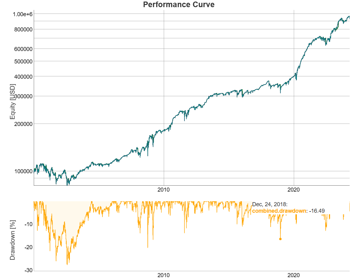
Here’s the performance with 1 tick slippage:

#Compute Backtest
BT%>%
  mutate(slippageTicks=1)%>%
  fComputePnL()%>%
  fCompoundPositions()%>%
  fComputePnL()%>%
  fPlotInteractivePerformanceChart()

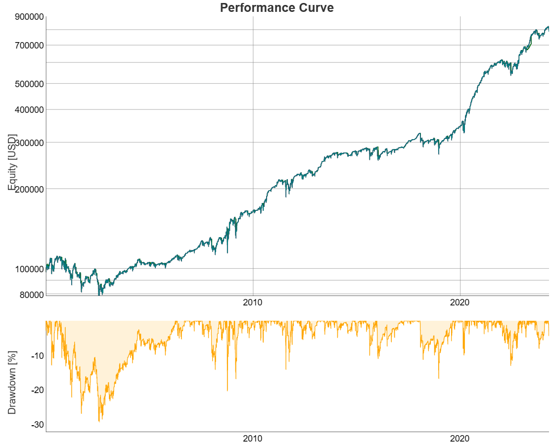
And with 2 tick slippage, to check the magnitude of the edge:

Still positive.

Now let’s try a different IBD range, with 1 tick slippage. Enter Long when IBD<0.15 and Exit when IBD>0.85.

It holds up. Overall not bad performance for such a simple strategy.

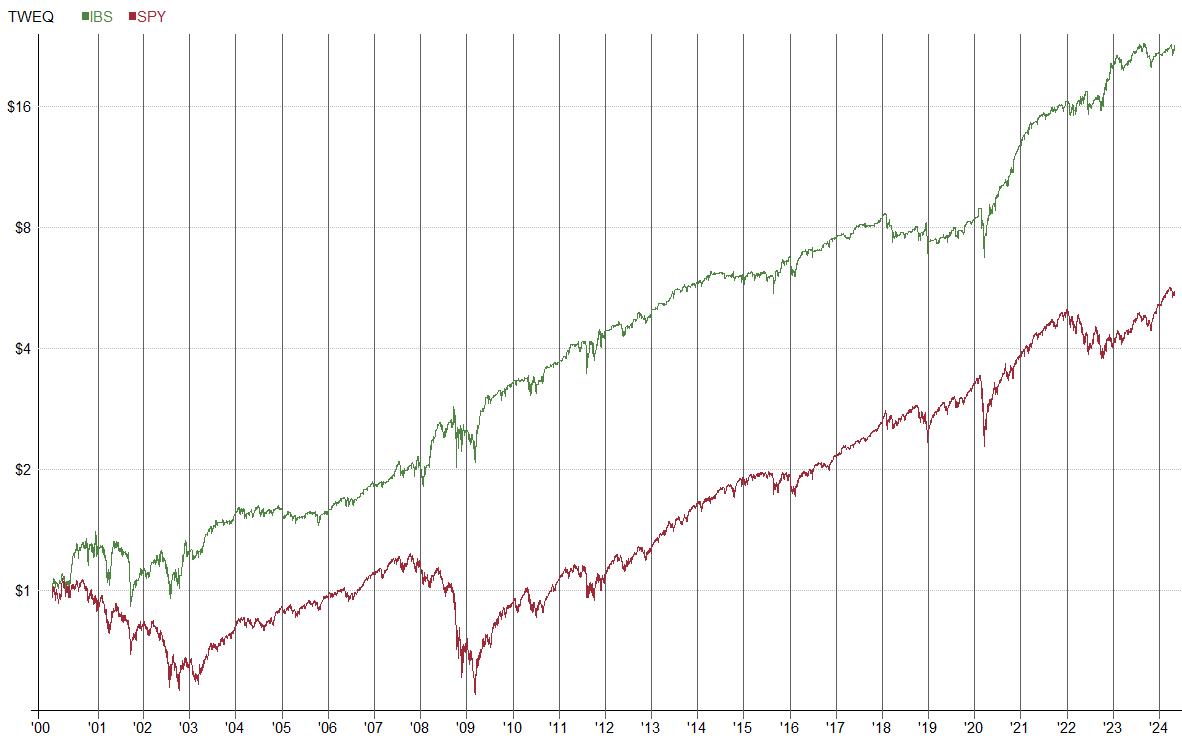
Now let’s test a similar strategy in RealTest, which trades SPY, QQQ, IWM and DIA ETFs, also with 1/N sizing and IBD>0.2 entry, to double check:

Looks OK. Now…. note there is a relatively high correlation to S&P500

What’s next? To do similar analysis into different technical analysis indicators (RSI, etc..) and rules; and come up with a collection of technical analysis trading strategies.

These strategies which work in a few markets but fail in the rest, without a fundamental economic reason for doing so, are less robust and more prone to be random. The solution? To stack together a lot of these weak edges and watch closely over time. Trade with paper trading account for a few months before going live, to remove the crappy ones, then kill the ones that turn out to be random after a few months of live trading. And allocate less capital to these strategies than more robust strategies such as trend and carry.

This particular one goes to my strategy “incubator” in the paper trading account.

Lemme know what you think!