Setting up a Portfolio of Futures Trading Strategies
The holy grail of investing: Uncorrelated Strategies
Ray Dalio says the holy grail of investing is in trading multiple uncorrelated strategies. Diversification can be achieved by trading systems with different underlying principles, time frames and asset classes, over a wide range of instruments.
Following an ideas-first approach to trading; not trying to uncover patterns in the data but working with base principles. As per AQR’s definitions of style premia:
Trend: Tendency of asset recent relative performance to continue in the future.
Carry: Tendency of higher yielding assets to outperform lower yielding assets.
Value: Tendency of relatively cheap assets to outperform relatively expensive ones.
Defensive: Tendency for lower-risk and higher-quality assets to generate higher risk-adjusted returns.
I’m exploiting these base principles (so far) using several daily timeframe strategies:
[Trend] Trend Following: Long/Short momentum on equities, currencies, commodities, fixed income, rates.
[Carry] Carry: Long markets in backwardation, short markets in contango. Confirm with short term momentum.
[Carry] Curve Carry: Calendar spreads on commodities, exploiting the change in curvature of the term structure for each contract as contracts move towards expiration.
[Carry] Futures Contract Expiration: Long/Short cash-settled contracts when close to expiration, as the futures price converge to spot.
[Carry] VIX Basis: Exploit the VIX term structure. Short VIX futures (sell volatility) when contango. Long VIX futures when backwardation.
[Value] Relative Value: Exploit price relationships between commodities and stocks (producers, processors/refiners).
Asset Allocation: Vola risk parity long-only portfolio of stock index, bond and gold.
Strategies Performance
All the above strategies are implemented with Futures, except the relative value one, which trades stocks. The above strategies don’t deliver a great risk/reward individually but the combination does.
Let’s see how the individual strategy performance looks like:
It’s hard to compare individual strategy performance properly, since each one has a different leverage. Let’s normalize the strategies to 12% volatility for comparison, for apples-to-apples comparison.
Here we multiply the position allocations by these factors to get the same leverage in each strategy:
Overall positive, with each strategy doing its own thing, with some sizeable drawdowns every so often. The asset allocation “risk parity” strategy got hammered badly twice since 2020, as the equity and fixed income correlation character changed. Now let’s evaluate the historical correlations of the strategies. We expect low correlations since we are attacking the markets from different angles, timeframes and instruments:
Yearly rolling correlations look decent overall. Except for asset allocation and trend following, which oscillate around +/- 0.5, since trend following portfolio periodically gets concentrated with long bonds and equities.
Let’s check what happened during the 2007-2009 global financial crisis, and during the Covid crisis of 2020.
Correlations remained low, or changed gradually during the GFC which is interesting. During Covid crisis a sharp change of correlations is seen across several strategies. Notably the VIX Basis strategy switches from short volatility to long volatility in March 2020, which offsets the losses during the crisis in the asset allocation strategy.
Combining the Strategies into a Portfolio
How much to allocate to strategies at any given time depends on the correlations, volatility, expected returns, and an assessment on the robustness of the strategy.
Let’s try out different methods: Naive 1/N allocation and risk parity: volatility, correlation, and volatility + correlation.
Naive 1/N portfolio allocation
Let’s allocate 1/7th of the portfolio principal to each strategy at any given time, meaning each when a new signal comes, the strategy would size the orders using 1/7th of the principal.
Note I’m talking about the “dry powder”, which is your account net liquidation value minus open profits/losses. This is to avoid pyramiding.
Net Liquidation Value = Principal + Open PnL
OK, here we go:
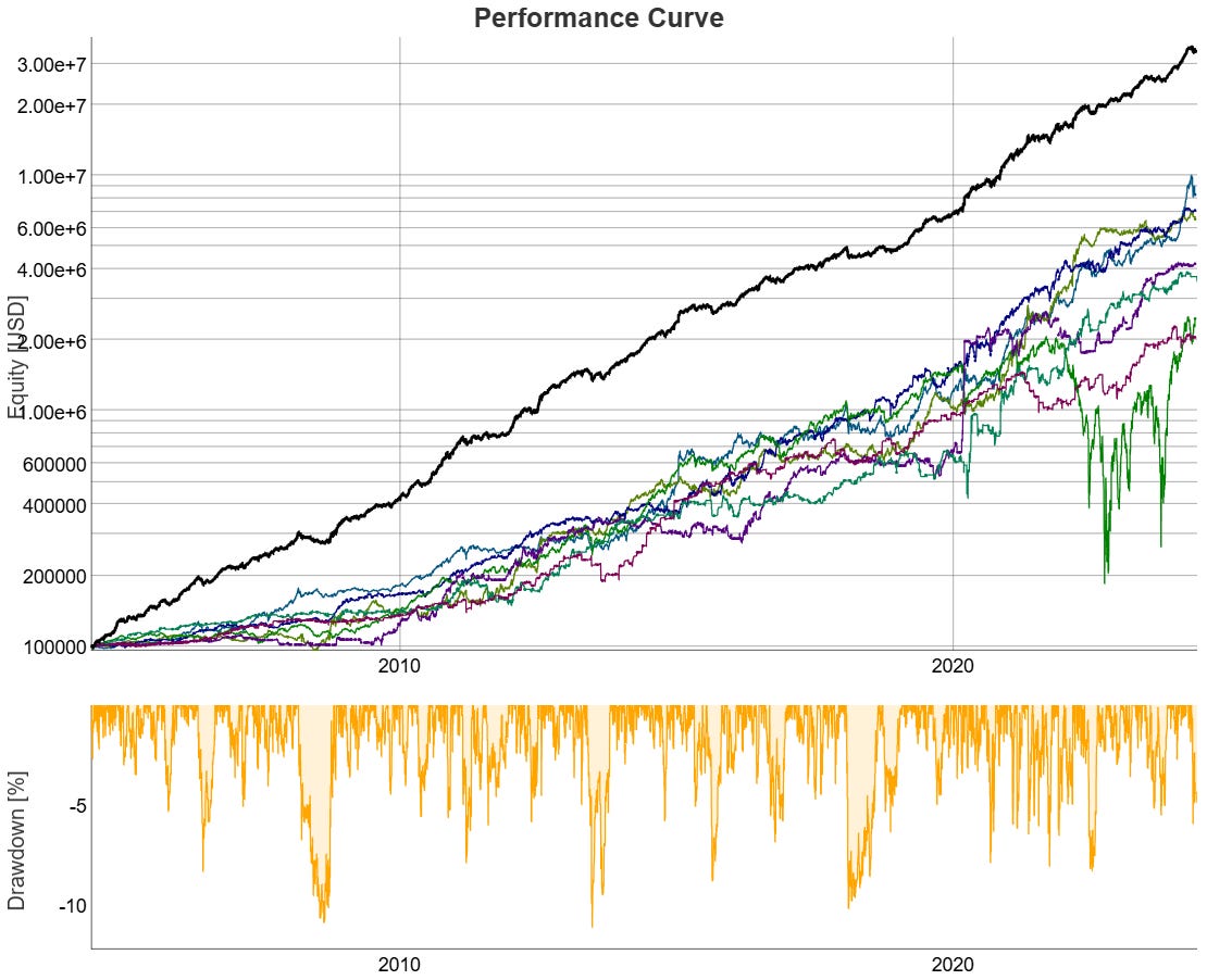
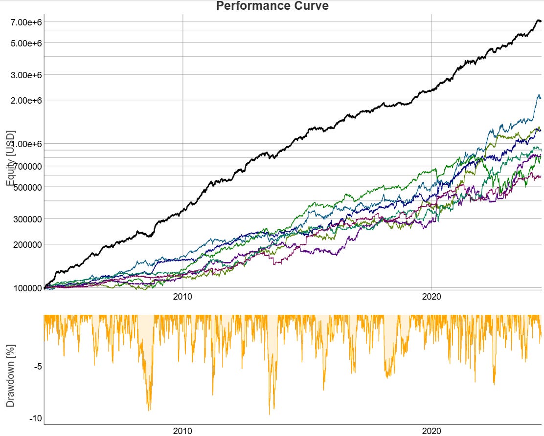
The chart shows the portfolio performance in thick black line, and the contributions for each strategy to the portfolio performance.
That’s a CAGR of 16.7% with historical drawdowns of <6.2%. Looking pretty good.
Note how during drawdowns, some strategies can lose most or even more than the money they made historically up to that point. This is because we progressively increase the cash allocated to each strategy as our portfolio value increases.
Historical drawdowns are manageable. Let’s leverage the strategy 2X and see how it looks:
A CAGR of 33% and max historical drawdown of ~11.2%. Here we assumed 1 tick slippage for each trade (outright or calendar spread leg). Rolls are assumed as 2 trades, but in practice I use calendar spreads for rolls, to reduce slippage. Let’s double the slippage assumption and see how it looks:
CAGR decreased to 30% and drawdown increased to 12%. This will be our reference case from this point onwards.
Volatility Risk Parity (VRP)
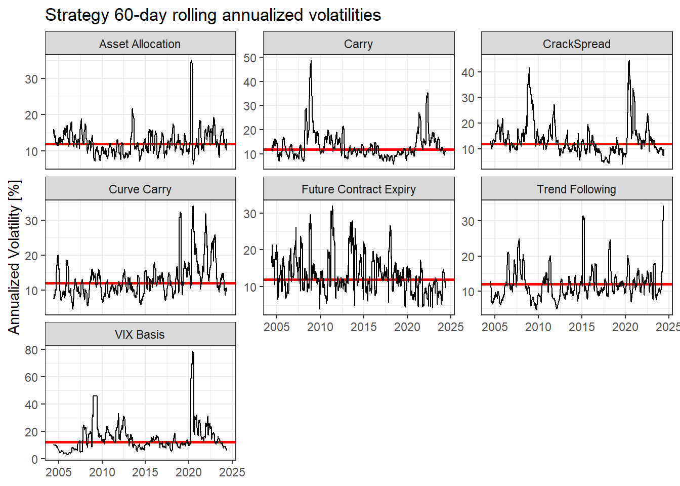
Let’s now try adjusting the position sizes based on the volatility of the equity curve of the individual strategies. Daily volatility is estimated as the standard deviation of log returns over 30 days, and annualized by multiplying by squared root of time. 1 year has ~256 trading days, so we annualize the daily volatility by multiplying by 16.
annualized_vola=roll_sd(ln(vami/lag(vami)),width=30)*16*100
Note how the volatilities go all over the place for the “Future Contract Expiry” strategy. This is because we only hold positions for short period of times, and trades are clustered around mid-month or end-of-month. So we’ll just use a fixed number of 12% for volatility of this strategy and use the actual estimated volatility for the rest.
OK, now we have to convert the volatility of each strategy to a scaling factor, such that the sum of the scaling factors is equal to 1. For the previous naive 1/N allocation we had a fixed allocation of 14.29% for every strategy (1/7), but in this case the allocation of each strategy will change over time.
Important note: no vola adjustment for open position for trading strategies, except for the asset allocation strategy during rebalances. Let’s see how the volatility risk parity allocation impacts or base portfolio:
The average drawdown is reduced to 9.7%, and the CAGR is reduced to 25%. There is also a wider dispersion in the strategy contributions. Looks encouraging.
Correlation Risk Parity
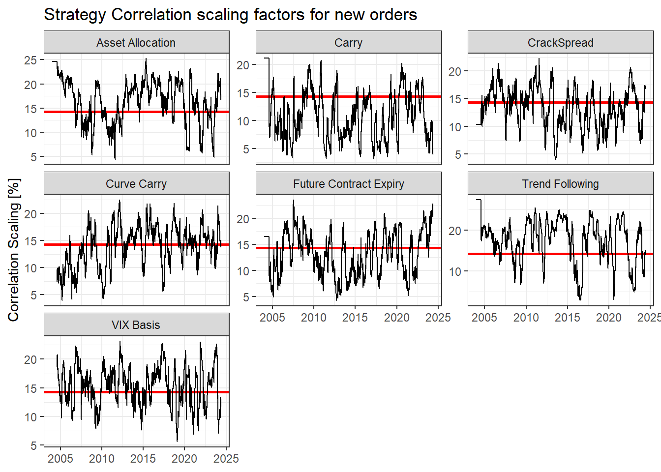
OK, now let’s see how it looks if we scale the entry order sizes based on the pairwise correlations. We do it like this:
Get log returns time series for each strategy.
Arrange log returns for each strategy pair.
Compute 90-day rolling correlations for each strategy pair.
Compute the scaling factor using Gaussian scaling, for each strategy and date:
(each strategy and date would have 6 rows. Corresponding to pairwise correlation between the given strategy and the other 6; 42 rows per date)
Where:
𝑍 is the Z-score.
𝑋 is the pairwise correlation
μ is the mean of the correlation matrix
σ is the standard deviation of the correlation matrix.
Now, for the performance, scaling entry sizes by correlation only:
We get a CAGR of 27% and max drawdown of 12.6.%, with an overall wider dispersion on the individual strategy contributions.
Volatility + Correlation Risk Parity
OK now let’s try to adjust by both volatility and correlation. Let’s compute a combined scaling factor which weighs 50% to inverse volatility and 50% to inverse correlation factor, then scale it so it sums to 1 for the portfolio.
Interesting… it looks very similar to the Naive 1/N base case.
Let’s check the performance of the combination:
OK, CAGR 26% with max drawdown 10.7%. The added complexity doesn’t hit the ball out of the park!.
Other portfolio management ideas to try, later on
Equity Curve Trading: Enter/Exit the strategy based a criteria. For example 200-day moving average or more advanced regime filters.
Martingale: If we assumed every strategy is robust and will recover from every drawdown, we can allocate to strategies following the “Martingale” method, where we put more capital during drawdowns (up to certain level), and less capital during equity highs.
Other advanced asset allocation methods.
Portfolio comparisons
Let’s summarize our observations into a chart and a table:
It looks like the volatility risk parity improves performance a bit, and removes some outliers on positive and negative side.
But there is a key downside of volatility risk parity (in my particular context): reducing the leverage in strategies in a relatively small account can prevent from opening positions because it would require to buy less than 1 contract sometimes. This can happen in the Naive 1/N allocation also, but less often. Careful simulations are required to evaluate the impact of missing some trades and rounding position sizes.
Overall there is a huge positive impact in trading multiple strategies. Note how the Sharpe ratio of the portfolio is much larger than the Sharpe ratio of the individual strategies. So we are moving in the right direction.
Conclusions
Keep-It-Simple. Use 1/N strategy allocation, or a fixed allocation setting based on the conviction on the robustness of each individual strategy. Unless you manage a large pool of capital, where volatility targeting the porfolio makes sense.
Focus on developing more uncorrelated strategies with different:
Asset classes (equities, commodities, fixed income, rates, crypto)
Instruments: Futures, Equities, Crypto (spot & futures)
Styles: Trend following, mean reversion, carry, relative value
Timeframes: Long Term, Short Term
Directions: Long + Short
What’s next?
To research other strategy ideas for futures:
Add synthetic instruments, such as popular calendar spreads (with economic sense) to existing (or new) strategies.
Short term mean reversion.
Additional relative value trades.
Feature engineering (COT report, term structure, etc.) and machine learning model to predict next week’s market direction.
And away from futures:
Mean Reversion in stocks & crypto.
Trend following in stocks & crypto.
Stock Pairs trading (easy to execute but very hard to find the best pairs to trade).


Great article! Reminds of Rob Carver’s Advanced Futures book. In practice, adjusting the leverage/volatility with that precision would require a lot of contracts… tens of millions of dollars. He makes this point in his book
Great article! Whould you mind to share any more info on the strategy [Carry] Curve Carry: Calendar spreads on commodities?