Practical Diversified Trend Following: Deep Dive

Can Retail Traders afford this great strategy?

The intention of this post is to explore various aspects of diversified trend following strategies, and gauge how retail traders with modestly sized portfolios can trade this strategy. Get your coffee ready because this is a long one.

Trend following is recognized as one of the most robust trading strategies. Meaning you know it will make money in the long run. But with robustness comes pain and long drawdowns. One of the reasons cited for why this strategy works is precisely because it’s painful to trade.

Institutional allocators typically struggle to justify any meaningful allocation to this strategy beyond 5%, even though it is well known that >30% allocation against a 60/40 portfolio is optimal.

The solution to the pain is to trade more uncorrelated strategies. The more the merrier. There’s a catch though… how much capital you need to do this (?) We’ll explore this aspect.

There’s a few schools of thought in the trend following arena, which can be grouped around 2 main philosophies:

• Classic: Entry and trailing stop, or channels. Long/short. Same rules long & short. Take every trade. Size position at entry, with no adjustment thereafter.

• Modern: Dynamically adjust position sizes for changing volatility and correlation of each market; and portfolio. Scale positions based on momentum scores. Volatility target portfolio.

The classic one is a more divergent type strategy with positive skew. The other one is more neutral skew as it dynamically reduces sizes in big winning positions.

In addition, some traders advocate to trade every market they can get their hands on. Others prefer to trade a fixed subset of markets. There are successful traders in all camps, which shows that there are lots of different ways to go about trend following.

It has been mentioned by several traders historically that you need >1MM USD to trade a diversified trend strategy with futures. We need to explore this again in 2024, as there is now a wider selection of smaller futures contracts that retail traders can access (CME micros / minis, and a few markets in European and Asian exchanges). The challenge for traders with smaller accounts is that they need to round position sizes, so they can’t get the fine control on position risk that institutions can afford. For example, you want to hold 1.7 contracts for each 100K USD account. If you have 1 MM$ you would trade 17 contracts. With a 100K$ account you would round it to 2 contracts. Now… how much difference does this make? Let’s explore.

In my view, traders with limited capital looking to trade multiple strategies would have to hold less & larger positions, as opposed to more & smaller positions, to be able to trend follow with futures. It’s a downside for the small trader. On the flip side, the small trader can trade less liquid markets which the large institutions can’t.

So our goal is to maximize risk adjusted returns, while (for the smaller trader) constraining the number of open positions in order to allocate more risk per position and be able to afford more markets.

Some ways to reduce the number of positions:

• Set position count caps:

  • Rank new setups in ascending order by ATR*Point Value, or by a momentum score. Take entries until all the available position slots are filled.

  • Kick out poorly performing positions to make room for new entries. This increases the turnover significantly, but may pay off..

• Long biases, or removing sectors.

In the next sections we will explore different ways to go at trend following, starting from data, strategy design, then assessment of performance for different account sizes.

Data

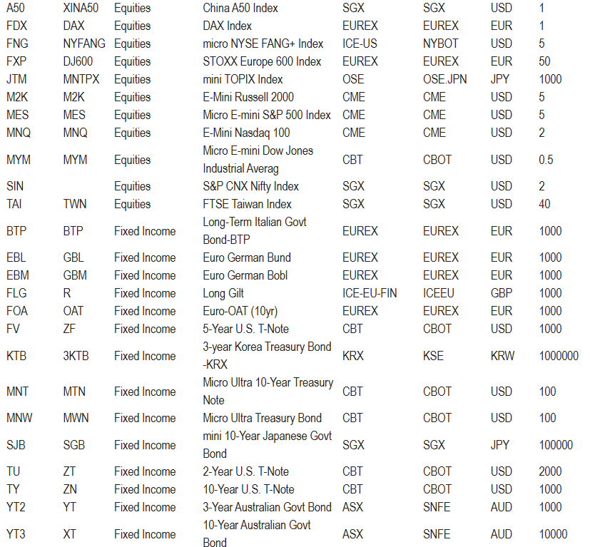
Let’s examine a universe of ~100 futures markets, out of which 10 are micros and minis, so 90 markets effectively. I use CSI Data as the sole data source for this study.

This is the list of markets:

Note some markets are currently delisted. Some markets are recently listed. Some are liquid and some illiquid today.

Futures contracts expire, so to facilitate the simulations, we stitch together the contracts into back-adjusted time series. I do 2 different back-adjusting of the data:

• Price-based adjustment; “Panama-Canal”.

• Returns-based adjustment.

Contracts are switched when the open interest of the back contract is higher than the front contract.

This is an example of continuous futures time series for a given market:

The “Panama Canal” method preserves the actual price changes of the individual contracts. The proportional method preserves the returns of the individual contracts. Note how the price-based adjusted (Panama Canal) time series can go negative in markets with historically positive carry (backwardation).

My simulation engine takes unadjusted, price adjusted and return adjusted series as input, in an R dataframe with columns such as:

symbol, date, delivery, nextdelivery, open, high, low, close, volume, oi, open.p, high.p, low.p, close.p, open.r, high.r, low.r, close.r

Where the suffix ‘.p’ is the price adjusted data, and the ‘.r’ is the returns adjusted data.

When the currently held contract open interest is lower than the next contract, the nextdelivery column will show the next contract, and the simulator will add commission and slippage for the corresponding roll-overs.

Contract selection criteria:

• For Fixed Income, Equities and Currencies, we hold the front or second contract; whichever has the highest open interest.

• For commodities and volatility, we hold the 2nd contract or later, whichever has the highest open interest. This is to remove some idiosyncrasies around commodity delivery, not have to worry about first notice day, and lessen the effect of carry on the trend signals (since I trade carry in a separate strategy). Front contracts in, say, natural gas have a stronger negative carry than the contracts farther away. See my post on commodities for more details.

• For deeply liquid interest rates, we hold the 8th contract onwards (2 years ahead in the future). As the front contracts have a low volatility and high tail risk.

Simulation

Classic Trend Following

Here’s a Classic “Loose Pants” Trend Following strategy:

• Rules:

  • Enter on 6-month high (for longs) or 6-month low (for shorts)

  • Exit based on 5-ATR trailing ‘chandelier’ stop and Donchian stop (rolling 2 month low)

• Fixed fractional position sizing. Each position risks a fixed % of principal.

• Size positions at entry and keep fixed.

• Trade every liquid market. Every market we can get our hands on.

• Long + Short the same way in every market. Same rules.

• Take all trades (can end up holding lots of positions).

OK, let’s explore the strategy at high level, assuming we could afford every liquid market.

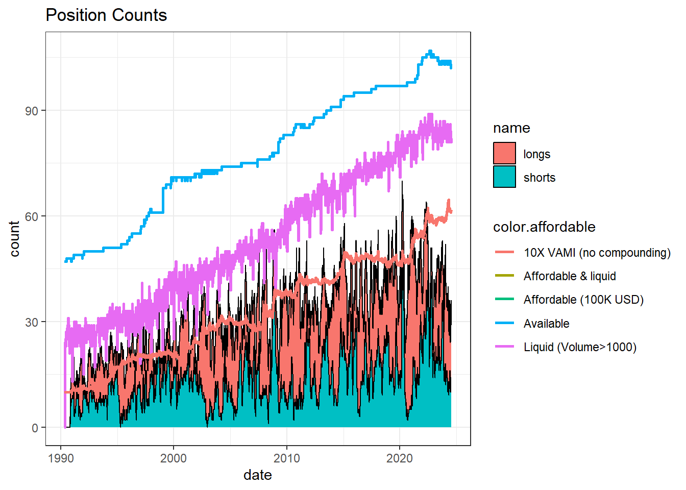
Note the number of open positions goes up as new markets become available for trading within our universe. Therefore we shouldn’t model taking the same position risk we use today for the past, because there were fewer markets before. The risk per position needs to be scaled down as the number of available liquid markets increase.

Let’s scale down the position risk at entry with the liquid market count.

OK this makes more sense. We start risking 1% of principal, and move progressively to 0.6% risk as more markets become available and more positions can be opened.

This is the equity curve:

The performance is in line with the TTU TF index, BTOP50 and SG Trend Index.

Source: TopTradersUnplugged.com

Dynamic Position Sizing

Using fixed position sizes can leave us with pretty large positions sometimes which would drive the volatility of the portfolio. This feature helps us make more money over the long run, but it’s hard to stomach, as it exposes us to quick and large losses when trends end.

adjust position sizes if target size is >50% off from the target size:

The performance looks visually similar.

The dynamic sizing logic will impact the outlier trades, which are the main driver of returns of the strategy.

Let’s check the impact of dynamic position size adjustment for the recent London Cocoa trade:

The size.c variable is the calculated size for the current volatility (ATR). The size variable is the actual position size we hold. The charts illustrates that fixed sizing ’Classic” system captures a larger profit in outlier trades. But can also incur greater losses. In the Cocoa example you can see the huge run and the large loss at the end for the fixed sizing, and a smoother (but less profitable overall) PnL curve for the dynamic position sizing. Fixed sizing is hard to stomach in outlier trades as the position volatility drives the volatility of the entire portfolio.

Limiting Entries

We can try to simply not enter a new position if we already fill a predefined position count limit. This would limit the number of trend opportunities we can catch early on. But big outlier trades would be caught on eventually, a bit later, as they keep making new highs (for longs), or lows (for shorts). This is what we’ll do:

• Rank all potential entries, “setups” by dollar volatility: PointValue * ATR. To focus on more ‘affordable’ liquid markets (like CME micros, for example).

• Setup a number of slots to fill. Let’s try 10,15,20,30 positions and compare results.

• First check for exits, to free the available slots. Then fill the available slots with entries.

Here is the analysis for multiple position counts, with leverage scaled to have similar median volatility, allowing for apple-to-apple comparison:

Surprise surprise. When normalized to the same leverage, we see the position caps of 10 and 15 positions for our futures universe actually improve performance. I think this is a pretty good insight for the smaller trader who can afford less positions than the institutions.

Assuming we could afford any market we wanted, what if we do the entry setup ranking using a momentum score instead? Intuition says that entering markets with more consistent trends (by whichever method used to quantify this) would improve performance.

Let’s try this one:

momscore=max(−2,min(2,0.42x0.456xEWMAC(16,64)+0.16x0.312xEWMAC(32,128)+0.42x0.212xEWMAC(64,256)))

Source: Derived from Robert Carver’s books and blog.

Interesting… There is a small improvement in ranking entries by momentum score vs. by affordability. Traders with limited capital can do the momentum ranking on the affordable markets only. More on this later.

Good. We are getting somewhere.

Kicking out poorly performing positions

Let’s try a variation of the entry limiting. How about we get rid of some of the worst performing positions to make room for new entries?

• Rank open positions by #ATRs drawdown from position high in descending order (highest drawdown on top).

• Kick out the worst positions, beyond certain drawdown score.

• Fill the available slots.

  AvailableSlots=PositionLimit−Exits−KickOutsAvailableSlots=PositionLimit−Exits−KickOuts

This increases the turnover of the strategy, but hopefully will improve the performance.

Observing the cumulative probability line, we can try kick-out thresholds for drawdown scores of 0.5 (kicks out bottom 25% of positions), 0.75 (kick outs ~10% of positions), 0.9 (kicks out <5% of positions). And let’s also simulate kicking out every position required to enter every new setup. The lower the drawdown score threshold, the larger the trade count and costs, so I don’t have an intuition of where this will take us…

Very interesting! Kicking out the worst performing positions (thresholds 0.5, 0.75, 0.9) reduces performance. Why this may be?

I think because it exits early some positions which would otherwise continue to be profitable, then you have to wait until hitting a new high (or low) to enter again.

However, if we make room to take every setup (threshold 0), the strategy becomes more profitable since 2008. This is surprising, because the increased trading costs would kill the performance in more expensive markets (larger spreads per volatility unit) such as interest rates, and in more mean reverting markets such as equities. That means that cheaper, higher volatility markets improved performance significantly. Using rankings for entries and exits (rotation strategy) is a different way to do trend following, which we will explore later in this post.

Long Bias

OK we’ve found that skipping entries improves risk adjusted returns and keeps position sizes in check, but kicking out poor performers to make room for more entries does not.

Our baseline strategy is now:

• Fixed fractional position sizing based on ATR.

• Adjust position sizes if target<0.5 x size, or target > 2 x size. (To sleep well at night).

• Trade every liquid market.

• Long + Short the same way in every market.

• Skip entries to control open position count.

Now it’s time now to analyze the performance attribution by sector and by trade direction (long vs short). These are the sector results for the “Loose Pants” strategy:

Alright. There’s a lot to unpack here:

• Around half the trades are shorts (see position charts in previous section).

• Shorts contribute negatively or little in Equities, Fixed Income, Grains, Softs, Metals.

• Shorts were profitable in interest rates after interest rates started to increase in 2020.

• Limiting entries changes the performance attribution, but the overall behavior is similar.

• Equity indices are less profitable than other sectors with these rules.

• Volatility and natural gas shorts are profitable, most likely due to strong negative carry, steep contango.

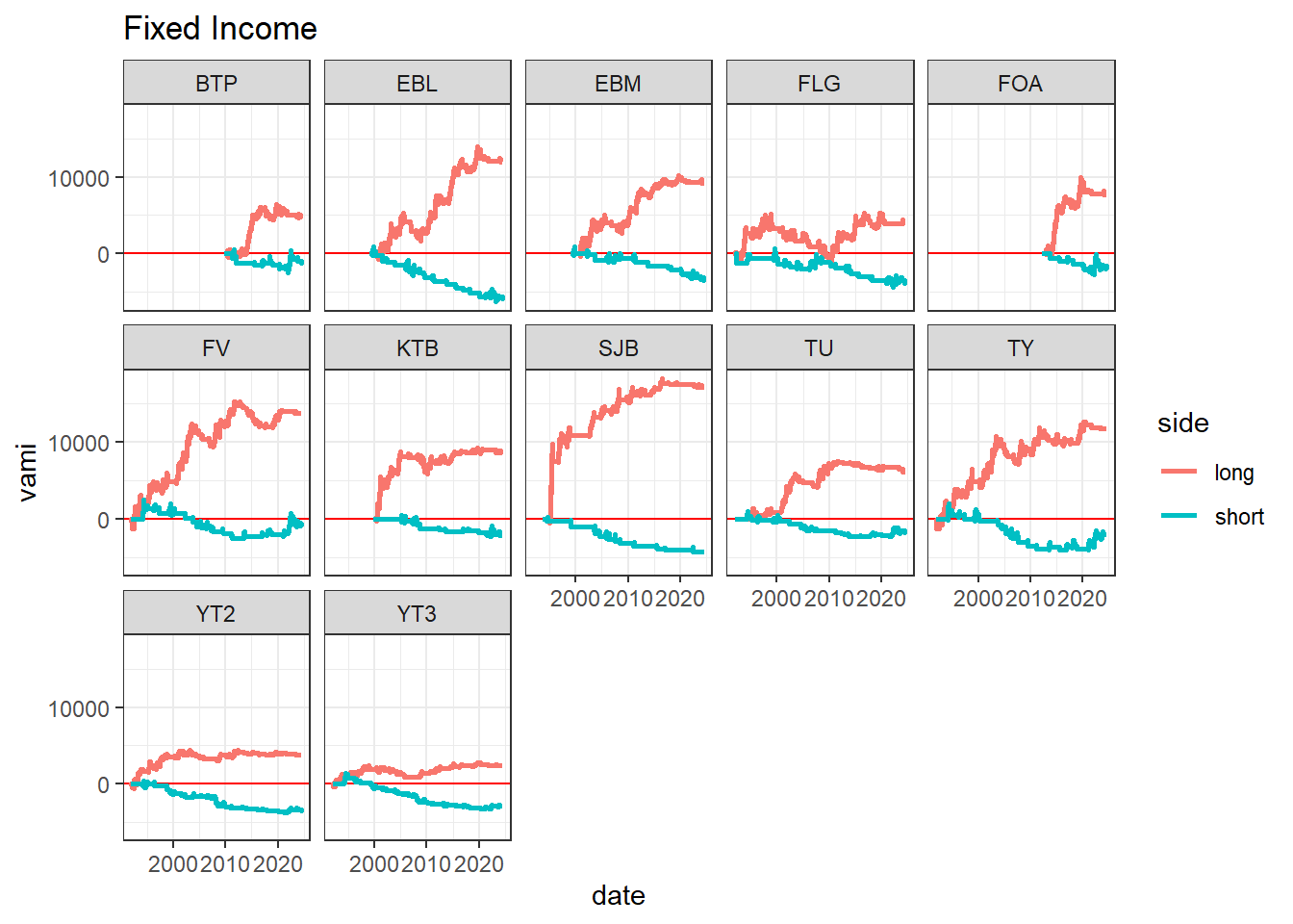
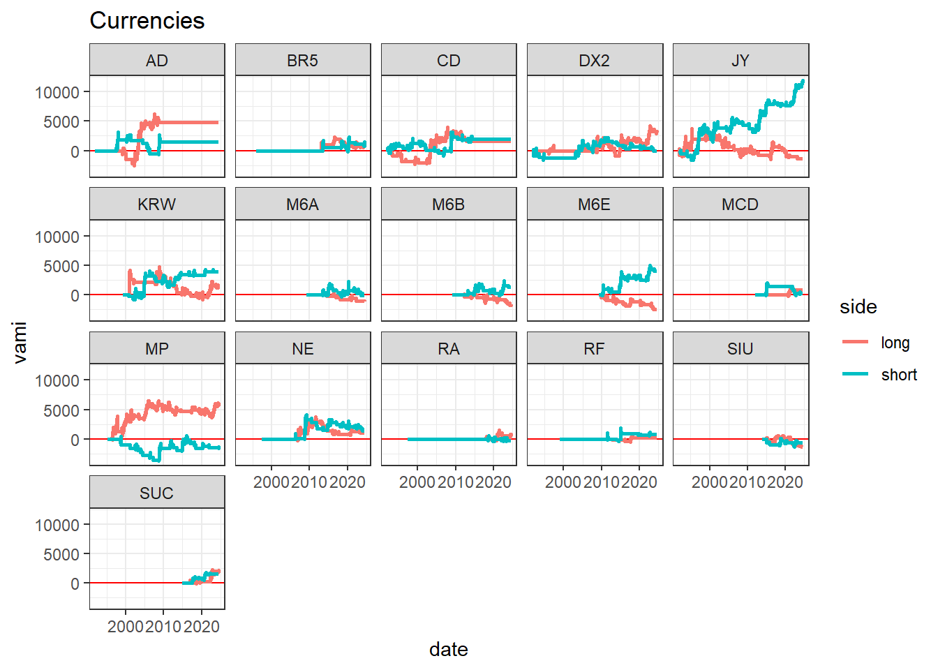
Let’s see market by market performance in our Loose Pants reference strategy to get additional insights.

Observations:

• Each individual market has a poor performance (crappy equity curves), but when stacked together in the strategy, the resulting performance curve is much smoother. Diversification at play.

• Some markets are unprofitable through their entire history, then the big profits arrive, such as Cocoa. I would not discard historically unprofitable markets, except for most shorts as they are consistently unprofitable over many uncorrelated markets.

• Several markets in universe are relatively illiquid.

Let’s check the impact of outliers in longs vs. shorts, for different strategy configurations:

It looks like limiting entries with momentum ranking improves profitability of shorts, but there are not enough big outliers in shorts to match the performance of longs.

OK now I will make a decision to get rid of shorts in Fixed Income, Equities, Volatility, Grains, Softs, Metals . The rationale, based on my context is:

• I already short volatility in other 2 strategies: VIX Basis and Curve Carry. Trend following would be shorting volatility most of the time, which would add too much exposure to volatility in my overall portfolio of strategies.

• Other strategies provide better profile for shorts. Better to invest my principal in those.

• I short interest rates already in the carry strategy.

• Equity indexes like S&P 500 are actually a slow momentum strategy (picks top N stocks by market capitalization, the ones which have outperformed, rebalancing quarterly), so shorting it is like betting against a momentum strategy. It wouldn’t make sense to me for a momentum strategy to short another momentum strategy.

• Fixed income shorts are consistently unprofitable for all the markets.

I will also get rid of volatility sector altogether, as I manage long volatility trades in the carry strategies.

The above decisions are debatable, but also note that I trade shorts in other strategies: Carry, Curve Carry, Mean Reversion, single ticker strategies, etc..

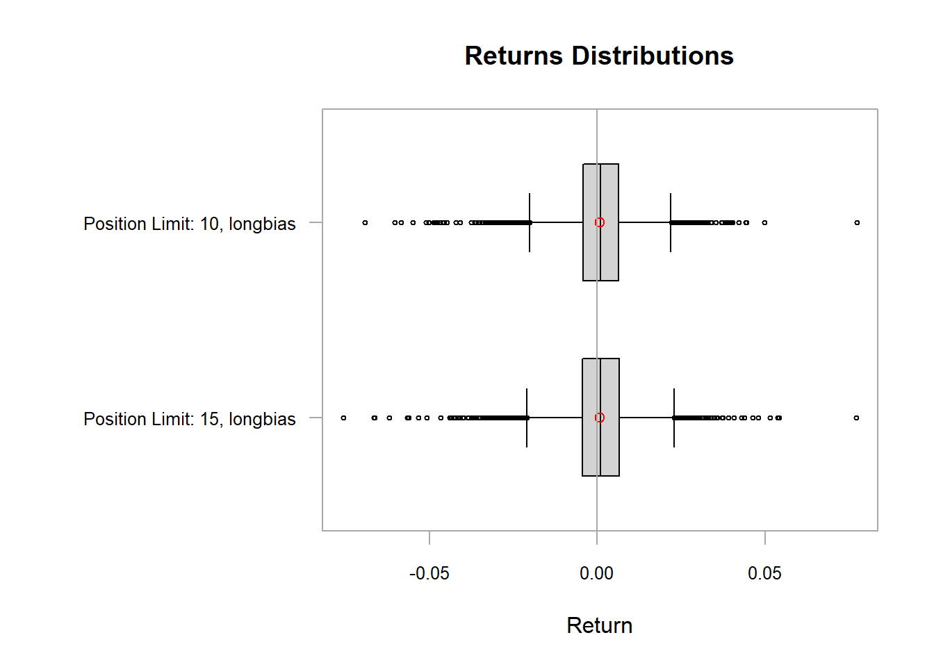
Alright. Let’s check the performance of the long biased, position-controlled strategies now:

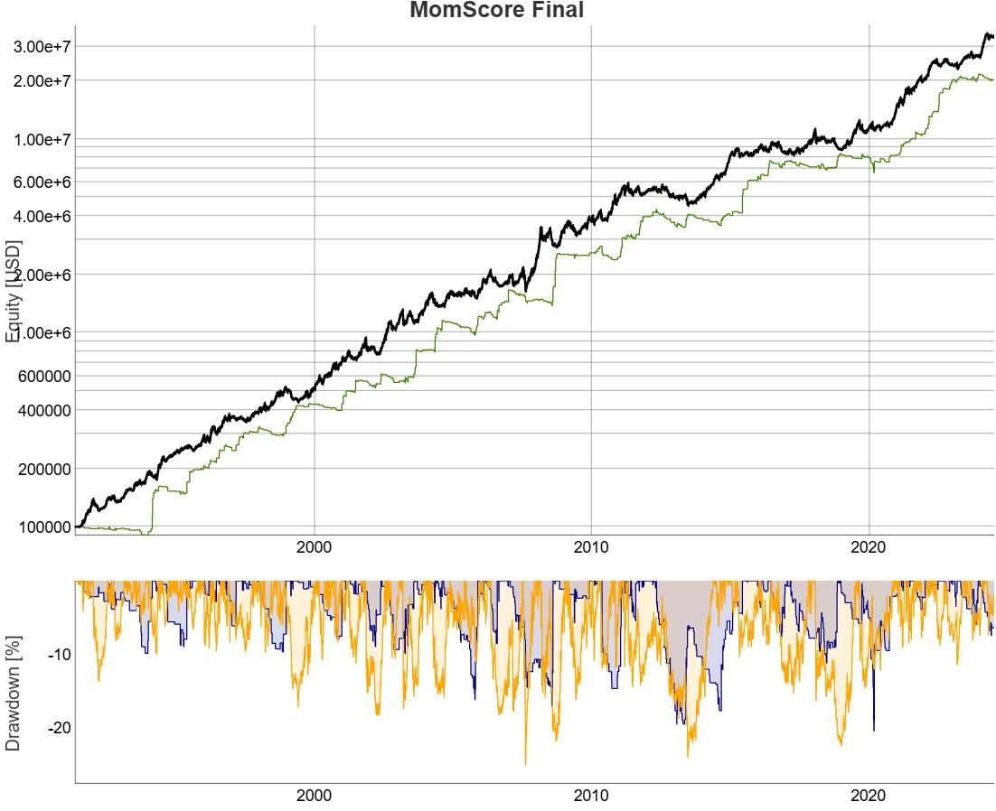
Performance looks better overall, with similar equity curves for 15 and 10 positions. This means we can capture the essence of the trend following returns with a smaller number of positions, which is great news for retail traders. Check out the performance curve.

Not bad for this “simple” system.

It told you it was going to be a looong article. Time for a stretch….

Continuous Trading System

A different way to do trend following is by continuous trading, without stop losses. Here’s what we will try:

• Compute several momentum scores.

• Scale momentum scores by their standard deviation. Cap to +/- 2 standard deviations to remove extreme values (which are possibly mean reverting).

• Simulate a strategy for each indicator, to enter long or short when |momentum score|>1 (a meaningful trend) and exit when momentum score changes sign.

• Run the strategy with the combined momentum scores using different weighing schemes. Decide way forward.

• Use momentum scores as scaling factor for position sizes.

• (Hopefully) The performance should be better and more robust with this added complexity.

Alright, let’s get our hands dirty. Here is the code to compute the momentum scores and scale them for 2 categories of momentum measures: returns over moving window, and exponential moving average crossover (similar to ROC and MACD respectively).

Now for the scaling…

The indicator distributions look interesting. The ewmac indicator looks similar to a normal distribution, and the lr looks like a triangular distribution. Now let’s simulate a strategy for each momentum score definition.

And the analysis performance of each momentum score, normalized to the same volatility:

Very interesting. Notice the dispersion of the performance with different momentum scores.

Now the ‘trick’ is to figure out how to combine the individual scores into a single one. Let’s keep it simple and assign a “U-shape” allocation to the 3 lookback of each of the scaled momentum scores:

This should be a good rule of thumb, as correlation of strategy returns between the short and long formation period is lower than the correlation of strategy returns between mid vs short and long formation periods. Note the other 3 indicators are variations of a single concept of calculated returns, so we can pick the best one. I like the “lr” (log returns) because the distribution looks more symmetric, but we have to check the performance to verify.

Let’s check 2 things:

• Performance of sizing positions based only on volatility.

• Performance of sizing positions based on volatility and the combined momentum scores. (Higher turnover but hopefully higher risk-adjusted returns).

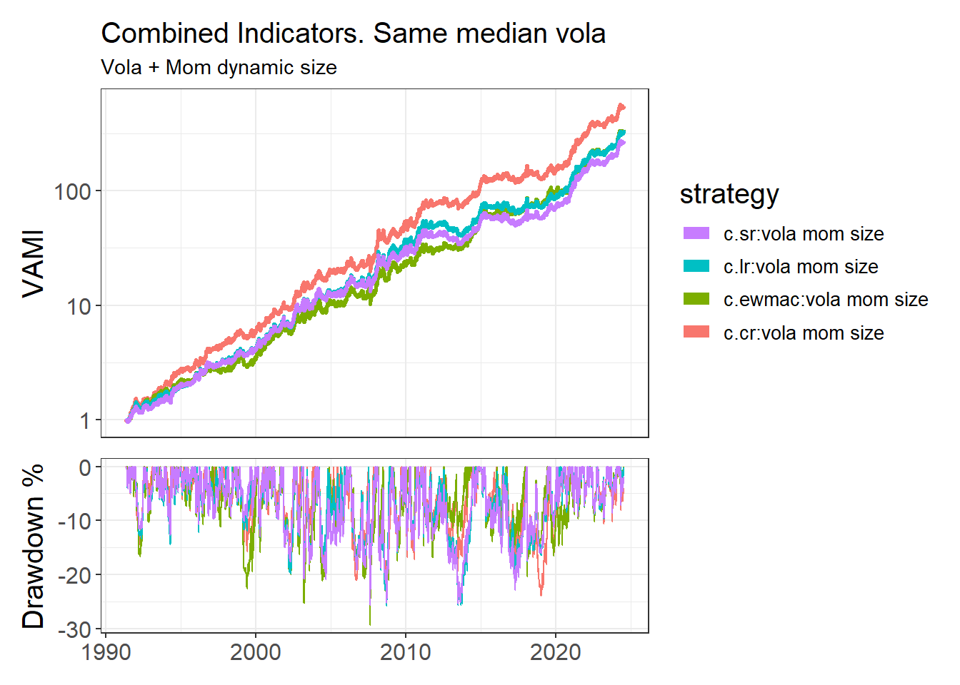
Here’s the performance of the combined momentum scores:

The way this strategy is configured, there is no additional edge in sizing positions dynamically using the momentum score.

Also it looks like the ‘cr’ (compound returns) score is a bit better than the others.

I would prefer to keep it simple and stick to the dynamic position sizing on volatility only. But for this article let’s go with sizing for vola and momentum, to demonstrate a “continuous trading” system.

Our resulting strategy, combining the ‘cr’ and the ‘ewmac’ scores 50/50, and dynamically sizing on vola and momentum is:

There’s no additional gain from the combining the two momentum scores into one. But we will still keep them combined. Here is the equity curve:

Looks nice. But it will be hard to afford for people with small accounts due to the large number of positions. Let’s limit the positions to 10:

The performance dropped.

One last attempt. Let’s use just the EWMAC score alone. I like it because anyways because it uses more data, vs. return based indicator which uses just a few points.

More research required into the interactions between the strategy moving parts which is causing such divergence in performance across momentum scores when capping position count.

Fascinating. With the EWMAC scores with 10-position limits, the character of the strategy has changed, and drawdowns are shorter. It doesn’t beat our (simpler) breakout with trailing stop strategy though.

Summary of rules:

• Compute momentum score with 3 lookback sets of EMA crossovers (ewmac).

• Scale momentum scores to a range of +/- 2.

• Enter when |mom score| >=1 (a meaningful trend). Exit when mom score changes sign.

• Dynamic position sizing on volatility and momentum, with 50% threshold (halve the size to reduce risk, double size to increase risk)

• Long bias: Skip Fixed Income, Equities, Metals, Grains, Softs sectors.

• No volatility sector

A Ranking System

Let’s re-use the same combined momentum score and structure the system in a different way:

• Every day, rank all markets by momentum score.

• If momentum score within top 7, enter.

• If momentum score outside of top 14, exit.

This system would hold up to 14 positions. Let’s see how it looks:

Very nice. It works also. A lot of additional research can be done on this type of system. I will leave it for other posts.

Combination of strategy types

What would happen if we trade the 3 trend following approaches together?:

1. Breakout with trailing stop

2. Continuous Trading System

3. Ranking System

Let’s check the correlations:

Pretty high correlations. So we don’t expect much gain from combining trend systems (which increases capital requirements, unless you trade fractional CFD contracts). Better to focus on creating other uncorrelated strategies (carry, mean reversion, etc.).

Anyways, here’s the combined performance with Naïve 1/N allocation across the 3 strategies:

As expected, some improvement (worth it still under some contexts), but not hitting the ball out of the park.

Summary of Strategy Design

• Explored 3 trend following approaches: Breakout with trailing stops, Continuous Trading, Ranking System.

• Checked performance attribution and decided to exclude shorts in some sectors.

• Compared performance of uncapped vs capped position count and decided to cap position count.

• Tested trading the 3 strategies simultaneously. Performance improved, but not game changing.

All the approaches are profitable. Given my personal context, up to this point (where we assumed we can afford everything), I’ll go with the simplest one; breakout with trailing stops. Summary of rules:

• Limit positions to 10

• Enter on 126 day breakout.

• Exit on 5 x ATR(20) stop or rolling 42 day low.

• Rank entry setups by momentum score. Note…it’s just a bit better than ranking by affordability. No major difference.

• Long bias: Skip Fixed Income, Equities, Metals, Grains, Softs sectors.

• No volatility sector

• Dynamically adjust position sizes when target size < 0.5 x current size or target size > 2 x current size.

Implementing the Strategy in Smaller Portfolios

OK finally we got to the main subject of the article. How much capital do we need to trade this stuff?.

CFDs

OK we got our reference strategy. Now let’s check the performance of trading it with expiring CFDs. CFDs are very heterogeneous. But let’s assume we can trade 1/5th of the futures contract for each CFD. Examining the IG Markets website, we can see that the spreads on expiring CFDs are much wider than in the futures. Let’s assume we lose 4 ticks per trade (entries, exits, rolls), for simplicity.

Note for trading CFDs, it is important to analyze properly the costs in detail with actual historical data. That requires another study in its own. A great resource overall to dig deeper into trend following, including implementation with CFDs is ATS Trading Solutions

The wider spreads heavily impacts the strategy, but it is still profitable.

Let’s check the performance using CFDs, for different account sizes. Assuming we cannot hold fractional CFDs (although in some brokers we can!). Due to differences in number of positions held, leverage factor is adjusted to achieve roughly 15% volatility.

We see that you can start trading a trend following strategy with CFDs with 25K USD, which is in line with capital requirements of systematic equity strategies. This is good because it allows sophisticated retail traders with access to CFDs to trade this strategy.

Futures

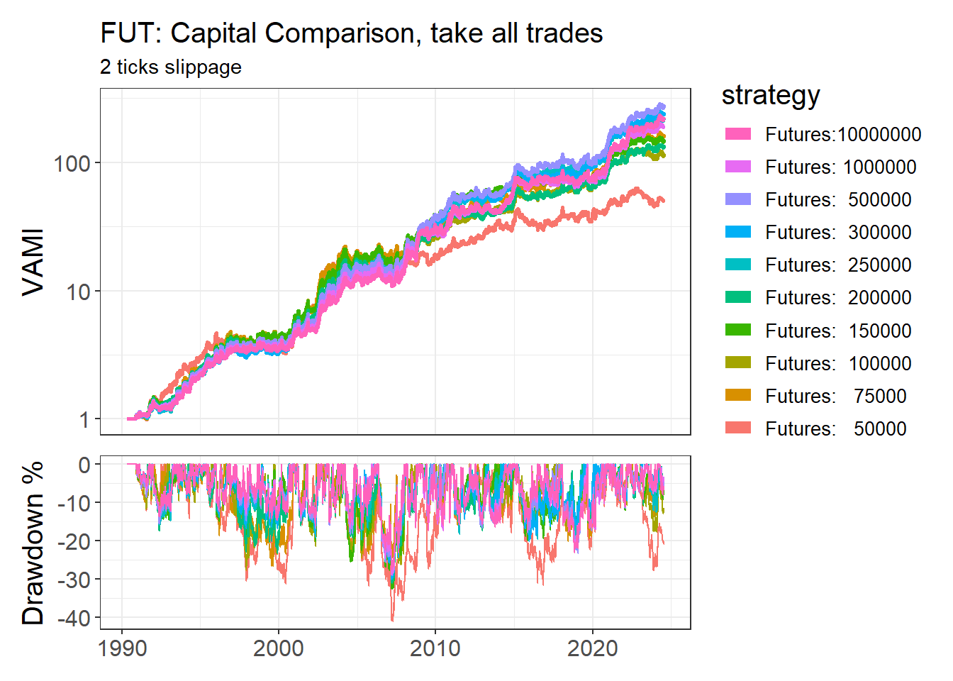
Now let’s check the performance using futures, for different account sizes. Due to differences in number of positions held, leverage factor is adjusted to achieve roughly 15% volatility.

Fascinating. We see at100K USD you can start trading a trend following strategy with futures effectively. This is much less than what is cited in different sources.

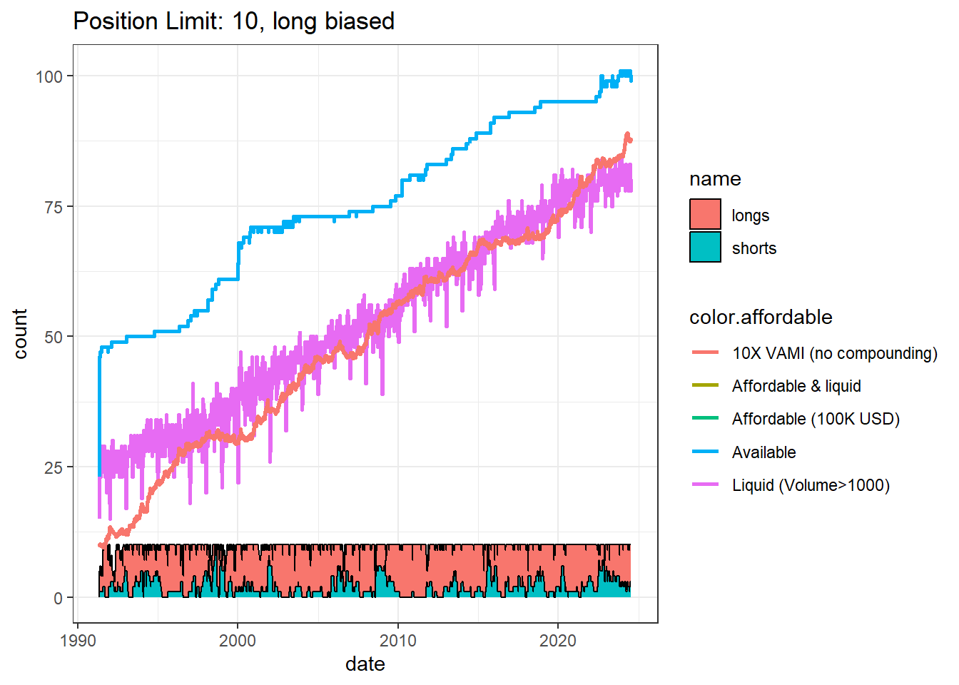
These are the position count charts for 100K and 1000K USD account for 10-position limit:

Interesting. Frequently we would hold less than 10 positions in the 100K USD case because of the smaller selection of available markets hence entry opportunities. Whereas for 1 MM$ we can access a lot more opportunities, so we hold 10 positions most of the time. But this does not make a noticeable difference in performance anyways.

One way to increase the number of opportunities is to relax the liquidity filter a bit. But this also means we would get markets with wider spreads which impact the performance.

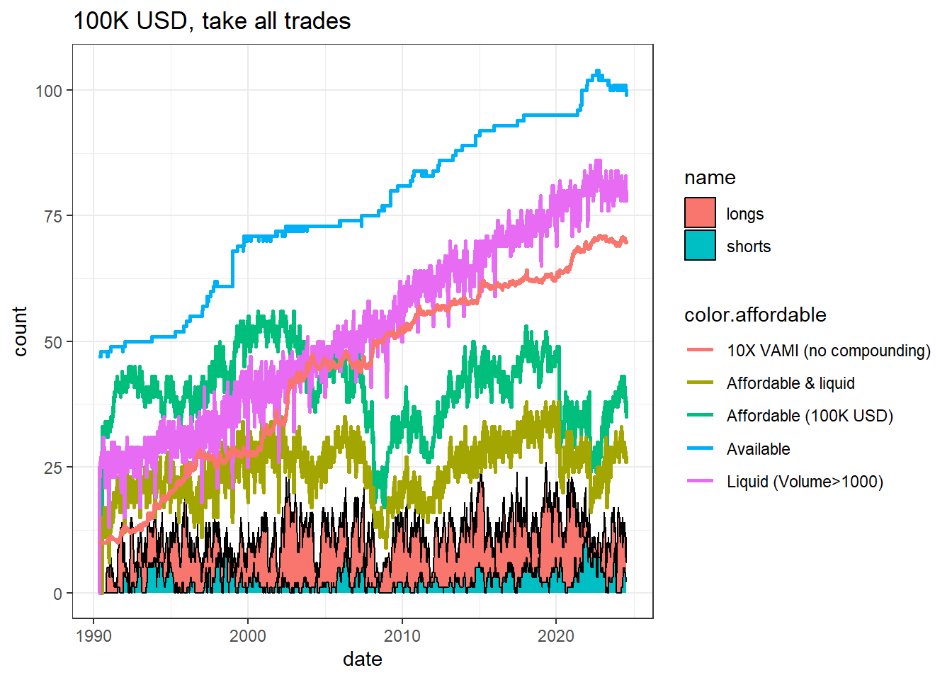
Another approach is to ditch the position count control altogether and go back to taking every affordable trade. Let’s test this:

We can reach a similar conclusion to the previous strategy. A minimum of 100K USD is required. Let’s check the position counts now:

For smaller accounts, the position count is kept under control because of the reduced number of affordable markets. The performance looks good as well.

Check out the list of positions for 29th July 2024, for the strategy which takes all affordable trades, by account size:

Pretty cool heh?

Execution Considerations

Execution is challenging because as you saw in the previous table, we are trading in exchanges all over the world, in different currencies, and in markets which have different opening and closing times, and different times in which there is a decent trading volume (liquid hours).

The data fetch runs at midnight New York time, while most US, Canada and European markets are closed. Strategy algo runs thereafter, and outputs a CSV file with the desired positions and sizes normalized to 100K USD.

An automated execution algorithm runs every 5 minutes for Interactive Brokers in an infinite loop, and does the following:

• Get the current net liquidation value (NLV…account size). Compare against a manually input reference NLV.

  • If deviation >2% between the reference NLV and actual NLV, the trader is informed via Telegram message.

  • If deviation>5% between reference NLV and actual NLV. The system does not place any order and the trader is informed.

• Current positions and orders in broker are compared against the expected positions and orders for the system. Sizes are computed based on the reference NLV.

• Difference between Broker and System orders & positions are summarized into a table of orders:

  • When we need to close one position and open a new one in a different delivery for a given market (i.e. rolls, etc.), a calendar spread order is submitted as a market order at the start of the liquid trading hours of the day.

  • Outright futures orders (not calendar spreads) are submitted using the Interactive Brokers patient adaptive algo at the liquid hours of the day, to try to get a better execution.

• Once every 2 hours, a Telegram message is sent to the trader informing that the execution engine is running (live check), and provides the current NLV.

I regularly check the execution engine is working as expected, and keep a record of the trades. The algo runs Python ib_insync library, wrapped in R using reticulate package. Integration between both languages works well.

Conclusions

This was a long article! I hope it sparks several ideas and discussions. Let me know if you find errors!.

Here are some conclusions:

• Yes, sophisticated retail traders can run a diversified trend following system with futures. But need >100K USD in capital to do so effectively with futures. Good news is that this is much less than what is often touted.

• Shorts are in general less profitable than longs except in high contango markets and in currencies (where longs and shorts are equivalent). I think it’s OK to skip the trend following shorts in some sectors to release capital other strategies which have better edges on shorts.

• “Loose Pants” vs. Other styles and variations of trend following: All profitable and valid.

• Trading all markets we can get our hands on vs. a limited portfolio: Both profitable and valid.

• Controlling position counts by limiting entries, vs. taking all the trades: Both profitable and valid.

• Combining different trend following strategies: Good idea, if capital available.

• Non-US residents with small accounts can use CFDs instead of futures. But need to study the costs, spreads and swaps (for cash CFDs) very well before pulling the trigger. Explore using mature CFD/Forex tools such as MT4/MT5 for easier execution. No escape from having to write a lot of code.

• Need an automated execution engine to trade this system plus other strategies effectively over multiple exchanges across multiple time zones. Unless you have time and dedication to place trade manually or semi-automatically.

Disclaimer

This article is documentation of research done by the author adapted to his own context. It does not constitute financial advice. Do your own homework.